EmbVision Tutorial: Part 2
Filtering and Frequency Analysis
Shogo MURAMATSU and Yuki TAKAHASHI
Niigata Univ.
Copyright (c), All rights reserved, 2014-2025, Shogo MURAMATSU
Contents
Summary
Through this exercise, you can learn 1-D signal filtering, frequency analysis and 2-D image filtering.
As a preliminary, close all figures by using function CLOSE
close all
1-D Frequency Analysis
First, load audio data "chirp" by using LOAD function for the following examples.
load chirp
The audio data is stored in variable y as a double precision array, where the sampling frequency is stored in variable Fs.
whos y Fs
  Name          Size             Bytes  Class     Attributes

  Fs            1x1                  8  double
  y         13129x1             105032  double
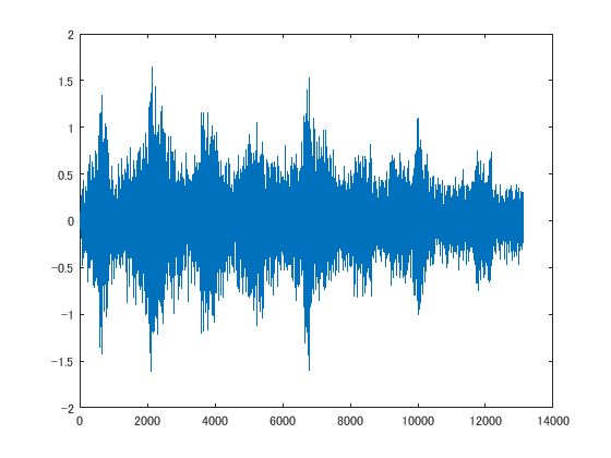
Next, load audio data "gong" and adjust the length by using LENGTH function to that of "chirp" and mixture them to produce another audio signal.
c = y; % Substitute y to variable c
load gong
g = y; % Substitute y to variable g

x = g(1:length(c))+c; % Adjust the lengths and mix the two audio data
Variable x stores the mixture audio data. Verify it by using PLOT function.
plot(x)
If audio is available, the audio can be played by using AUDIOPLAYER function.
First, create an audioplayer object.
player = audioplayer(x,Fs);
whos player
The audio is played by calling PLAY method of object "player."
play(player)
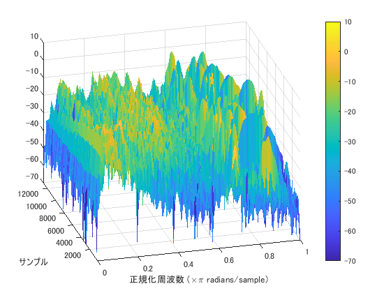
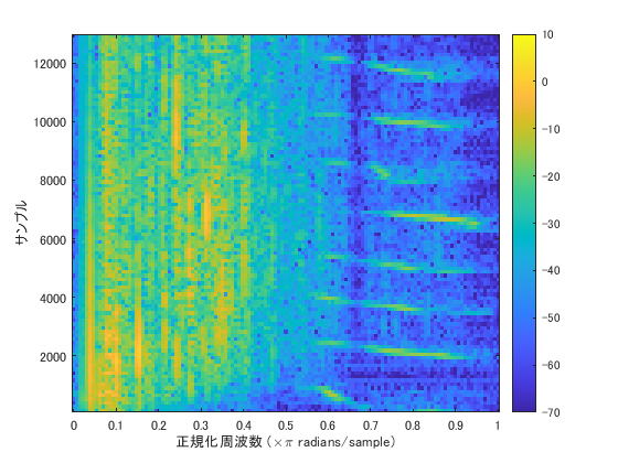
By using SPECTROGRAM function, one can analyze audio data through the short-time Fourier transform.
Under the condition
- Window length: 256
execute SPECTROGRAM.
figure(1)
spectrogram(x,256)
caxis([ -70 10 ])
colorbar
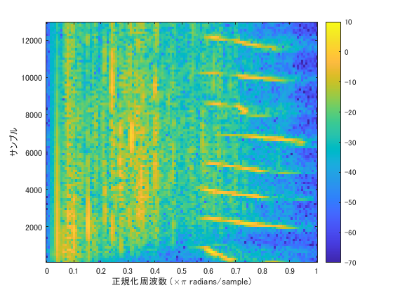
From the above command, a spectrogram, i.e., a time-frequency characteristic, of the audio signal is displayed, where the horizontal axis denotes the normalized frequency (  is normalized to 1 ), and the vertical axis is the sample indexes( the unit is
  second ).
Here, for the magnitude [dB] to easily be distinguished, CAXIS function and COLORBAR function are used.
Change the viewpoint with VIEW function.
view([-15 30])
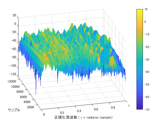
Adjust the range of the Z-axis from -70 to 10 by using ZLIM function.
zlim([ -70 10 ])
[ Top ]
Filtering of 1-D Signals
Next, apply linear filtering
![$$ y[n] = h[n] \ast x[n] = \sum_{k=0}^{N-1} h[k]x[n-k] $$](part2_eq02546691940298065541.png)
to audio data x, where the symbols are defined as
-
![$ x[n] $](part2_eq07825703633576993047.png) : Filter input,
: Filter input, -
![$ y[n] $](part2_eq10837726643215266746.png) : Filter output,
: Filter output, -
![$ h[n] $](part2_eq08380609512940977091.png) : Filter coefficients (impulse response),
: Filter coefficients (impulse response), -
 : Filter order.
MATLAB provides CONV function for the linear filtering.
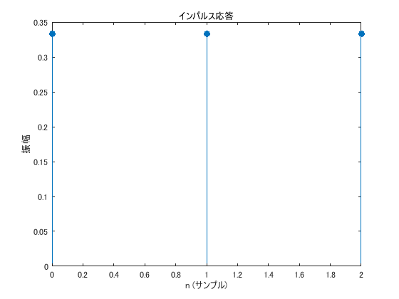
Execute linear filtering with the following filter coefficients.
![$$ h[n] = \left\{\begin{array}{ll}
1/3, & n=0,1,2 \\
0, & \mathrm{otherwise}
\end{array}\right. $$](part2_eq10275797988525623725.png)
h = [ 1 1 1 ]/3;
figure(2)
impz(h)
y = conv(h,x);
Variable y stores the filtering result. Verify the frequency characteristic (spectrogram) of output y.
figure(3)
spectrogram(y,256);
caxis([ -70 10 ])
colorbar
view([ -15 30 ])
zlim([ -70 10 ])
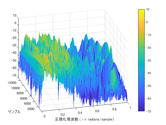
Compare the spectrograms of input x and output y. What would be noticed?
Observe the following characteristics:
- Frequency components higher around 4.0 in normalized frequency are attenuated.
- Particularly, high attenuation is observed around 0.667.
In order to verify the processed result by using audio player, execute the following commands.
player = audioplayer(y,Fs);
play(player)
[ Top ]
Frequency Response of 1-D Filter
Change of frequency characteristics through linear filtering is verified by frequency response of the filter.
Because the convolution in time domain is represented by
![$$ y[n] = h[n] \ast x[n] \ \stackrel{\mathrm{DTFT}}{\longleftrightarrow}\
Y(e^{j\omega}) = H(e^{j\omega})X(e^{j\omega}) $$](part2_eq00285256320026033444.png)
and it corresponds to the product in frequency (DTFT: discrete-time Fourier transform) domain, where the symbols are defined as follows.
-
 : Frequency characteristics of input ,
 -
 : Frequency characteristics of output ,
 -
 : Filter coefficients (impulse response) .
Frequency response of filter coefficients can be verified by FREQZ function.
figure(4)
freqz(h)
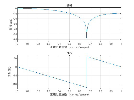
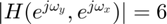
One can observe that the magnitude response attenuates over 6 [dB] for higher frequency than around 0.3 or 0.4. Particularly, the attenuation becomes large at 0.667.
Because
![$$ H(e^{j\omega}) = \sum_{n=-\infty}^{\infty} h[n]e^{-j\omega n}
= h[0]e^{-j0} + h[1]e^{-j\omega} + h[2]e^{-j2\omega} $$](part2_eq08621359951002256239.png)
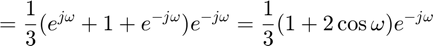
holds, the following properties can be understood.
-
 �ŁA
�ŁA 
-
 �ŁA
�ŁA  .
.
[ Top ]
2-D Frequency Analysis
Now, let us proceed to filtering for image data. As is for the previous audio data, linear filtering is available.
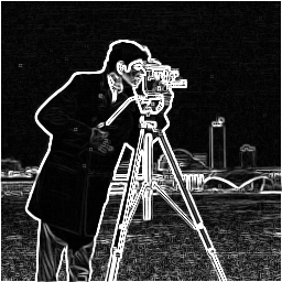
First, close all figures by using CLOSE function. Then, read prepared image "cameraman" and display it.
close all
figure(1)
X = imread('cameraman.tif');
imshow(X)
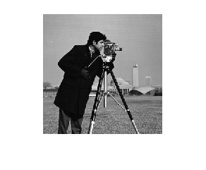
Image data is stored as variable X in 8-bit unsigned integer array. Convert this to double precision data.
X = im2double(X);
whos X
  Name        Size              Bytes  Class     Attributes

  X         256x256            524288  double
By using FFT2 function, one can analyze 2-D frequency characteristics of image data. Execute 2-D frequency analysis under the following settings:
- Point of 2-D FFT:

which is identical to the dimension of image X;
F = fft2(X,256,256);
whos F
  Name        Size               Bytes  Class     Attributes

  F         256x256            1048576  double    complex
Variable F stores the coefficients of the 2-D discrete Fourier transform (DFT). Because the results are obtained as complex data, take the absolute and obtain the magnitude.
Fmag = abs(F);
whos Fmag
  Name        Size              Bytes  Class     Attributes

  Fmag      256x256            524288  double
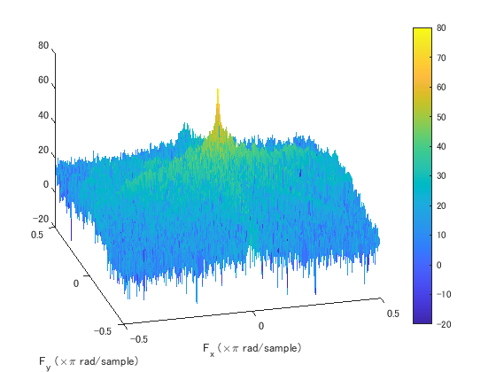
Variable Fmag stores real-valued array as the magnitude. Visualize the characteristics by using SURFACE function.
Prepare handle object hsrfc for adjusting the surface plot.
figure(2)
hsrfc = surface(20*log10(Fmag));
set(hsrfc,'EdgeColor','none');
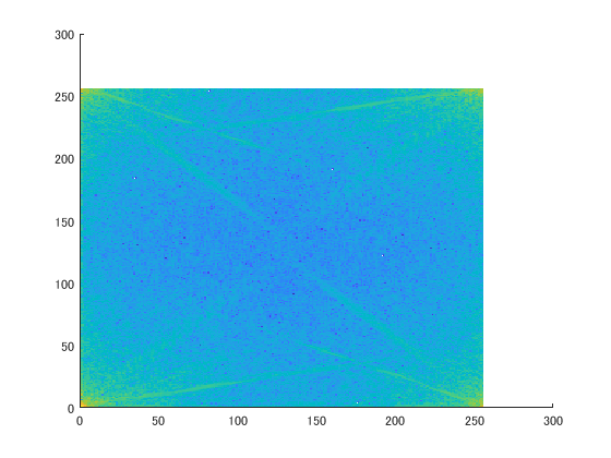
Note here that the results are recalculated as dB.
Put color bar for the sake of visual support.
colorbar
caxis([ -20 80 ])
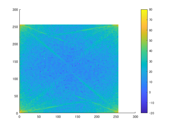
Shift the array by using FFTSHIFT function so that the DC component is located at the center.
set(hsrfc,'ZData',fftshift(hsrfc.ZData)); % Shift in the Z-axis
set(hsrfc,'CData',fftshift(hsrfc.CData)); % Shift in the component axis
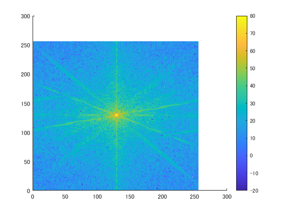
Adjust the coordinate for the normalized frequency representation.
fstep = 1/256; % Interval of frequency sample points
set(hsrfc,'XData',-0.5:fstep:0.5-fstep);
set(hsrfc,'YData',-0.5:fstep:0.5-fstep);
xlabel('F_x (\times\pi rad/sample)')
ylabel('F_y (\times\pi rad/sample)')
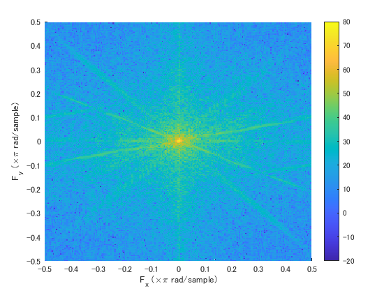
Change the view point.
view([ -15 30 ])
zlim([ -20 80 ])
[ Top ]
Filtering of 2-D Signals
Next, apply linear filtering
![$$ y[n_y,n_x] = h[n_y,n_x] \ast
x[n_y,n_x] = \sum_{k_x=0}^{N_x-1}\sum_{k_y=0}^{N_y-1}
h[k_y,k_x]x[n_y-k_y,n_x-k_x] $$](part2_eq18180359755469764686.png)
to image data X, where the symbols are defined as
-
![$ x[n_y,n_x] $](part2_eq03798263611009086944.png) : Filter input,
: Filter input, -
![$ y[n_y,n_x] $](part2_eq10019403117302485852.png) : Filter output,
: Filter output, -
![$ h[n_y,n_x] $](part2_eq12705266176939181025.png) : Filter coefficients (impluse response),
: Filter coefficients (impluse response), -
 : Filter order in vertical,
 -
 : Filter order in horizontal.
One can use CONV2 function or IMFILTER for 2-D linear filtering.
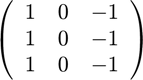
Execute linear filtering by using array
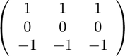
as the filter coefficients, .
H = [ 1 1 1 ; 0 0 0 ; -1 -1 -1 ];
Y = conv2(H,X);
Variable Y stores the filtering result, where the size increases 2 pixels in every dimension from that of original array.
size(Y)
ans =

   258   258
2-D linear convolution has a property that the output size becomes

when an image of size  is convolved with a filter of size
  .
.
Adjust the size of output image Y to that of input image X by trimming one pixel from top, bottom, left and right. It is convenient to use END function for the index.
Y = Y(2:end-1,2:end-1);
Output image Y may contain negative values as follows.
min(Y(:))
ans =

   -2.7882
Some treatment is required for the display as an image.
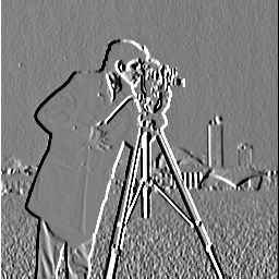
In the case of float type, IMSHOW function assumes that the pixel values are normalized to the range from 0 to 1. Thus, adjust the pixel values of output Y so that the negative values become less than 0.5 and positive values become more than 0.5.
figure(3)
imshow(Y+0.5)
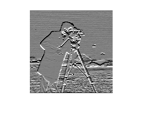
The previous filter produces a discrete approximation of vertical differential  .
.
Verify the frequency characteristics of output Y.
figure(4)
F = fft2(Y,256,256);
Fmag = abs(F);
hsrfc = surface(20*log10(Fmag));
set(hsrfc,'EdgeColor','none');
colorbar
caxis([ -20 80 ])
set(hsrfc,'ZData',fftshift(hsrfc.ZData));
set(hsrfc,'CData',fftshift(hsrfc.CData));
set(hsrfc,'XData',-0.5:fstep:0.5-fstep);
set(hsrfc,'YData',-0.5:fstep:0.5-fstep);
xlabel('F_x (\times\pi rad/sample)')
ylabel('F_y (\times\pi rad/sample)')
view([ -15 30 ])
zlim([ -20 80 ])
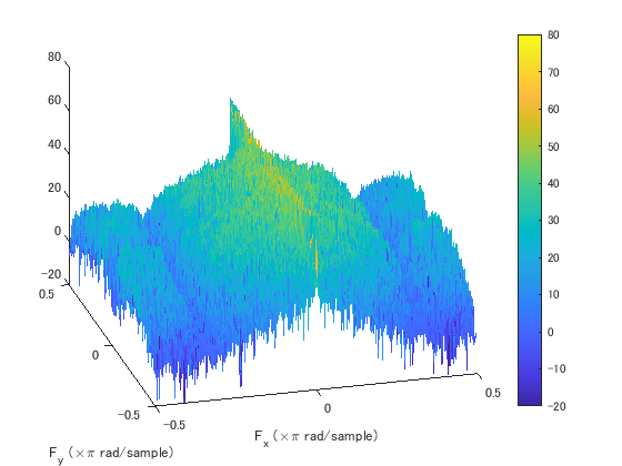
Compare the frequency characteristics of input X and output Y. What would be noticed?
Observe the following characteristics:
- DC peak was annihilated.
- Horizontal high frequency components were attenuated.
[ Top ]
Frequency Response of 2-D Filter
Similar to the 1-D case, change of frequency characteristics through 2-D linear filter is verified by the frequency response of the filter.
Because the convolution in spatial domain is represented by
![$$ y[n_y,n_x] = h[n_y,n_x] \ast x[n_y,n_x] \
\stackrel{\mathrm{DSFT}}{\longleftrightarrow}\
Y(e^{j\omega_y},e^{j\omega_x}) =
H(e^{j\omega_y},e^{j\omega_x})X(e^{j\omega_y},e^{j\omega_x}) $$](part2_eq14478578511036128230.png)
and it corresponds to the product in frequency (DSFT: discrete-space Fourier transform) domain, where the symbols are defined as follows.
-
 : Frequency characteristics of input$$ x[n_y,n_x] $$,
 -
 : Frequency characteristics of output ,
 -
 : Filter coefficients (impluse response) .
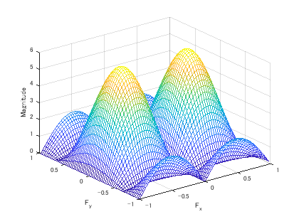
Frequency response of filter coefficients can be verified by FREQZ2 function.
figure(5)
freqz2(H)
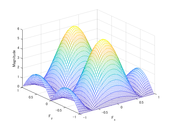
One can observe that the magnitude response attenuates the DC component and high frequency components in horizontal direction and has bandpass property in the vertical direction.
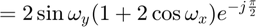
Because
![$$ H(e^{j\omega_y},e^{j\omega_x}) = \sum_{n_x=-\infty}^{\infty}
\sum_{n_y=-\infty}^{\infty}
h[n_x,n_y]e^{-j\omega_y n_y}e^{-j\omega_x n_x} $$](part2_eq06601985027195152832.png)

holds, the following properties can be understood.
-
 �ŁA
�ŁA 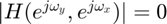
-
 �ŁA
�ŁA - At
 ,
, - At
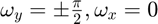 ,
, 
[ Top ]
Exercises
Exercise 2-1. Horizontal Differential Filter
Prepare the array
(discrete approximation of horizontal differential operation) as and apply the linear filtering with to grayscale image "cameraman.tif." Store the result to a TIFF file named "cameramangradx.tif," where the bias with 0.5 should be applied by taking account of negative values.
Verify also the frequency magnitude response of the filter.
(Example Answer�j
Exercise 2-2. Magnitude and Direction of Gradient
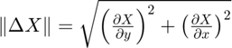
From vertical differential operation and horizontal differential operation  , Obtain
- Magnitude of gradient:
- Direction of gradient:
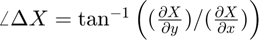 .
.
Then, store the results to image files "cameramangradmag.tif" and "cameramangradang.tif," respectively, where the direction should be normalized the range from 0 to 1.
(Example Answer�j