EmbVision Tutorial: Part 1

Image I/O and Pixel Processing

Shogo MURAMATSU and Yuki TAKAHASHI
Niigata Univ.

Image Read
Image Display
Array Operations
Pixel Processing
Image Write
Exercises

Summary

Through this exercise, you can learn how to read image files, display images, and write image files by using MATLAB. As well, you can also experiment simple pixel processing.

As a preliminary, close all figures by using function CLOSE

close all

Image Read

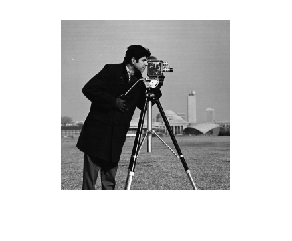
To read an image from a file, use IMREAD function on the MATLAB's command window with a file name as the argument.

I = imread('cameraman.tif');

Since cameraman.tif is a grayscale image, variable I is stored as a 2-D array.

If not specified, the data type becomes unsigned 8 bit ( UINT8 ) in default.

One can verify it by using WHOS function on the command window.

whos I

  Name        Size             Bytes  Class    Attributes

  I         256x256            65536  uint8

The size is displayed as height $\times$ width.

In order to verify the image size, SIZE function can also be used.

size(I)

ans =

   256   256

Set the second argument '1' in order to get the height.

size(I,1)

ans =

   256

Set the second argument '2' in order to get the width.

size(I,2)

ans =

   256

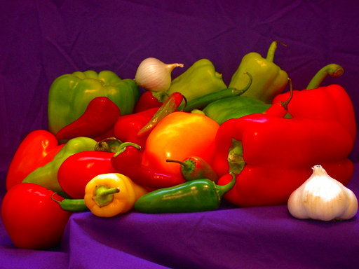
Color picture is also available.

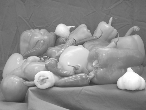
RGB = imread('peppers.png');

Variable RGB stores the pixel data as 3-D array.

whos RGB

  Name        Size                Bytes  Class    Attributes

  RGB       384x512x3            589824  uint8

[ Top ]

Image Display

MATLAB displays an array data as an image through IMSHOW function.

To display variable I as an image is as follows:

imshow(I)

Variable RGB is displayed by the following command.

imshow(RGB)

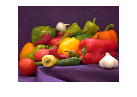
Then, a color image shows up.

[ Top ]

Array Operations

Image processing is executed by array operations.

First, we see some simple array operations. As an example, we'll use the following array.

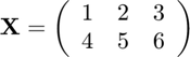
$\mathbf{X} =\left(\begin{array}{lll} 1 & 2 & 3 \\ 4 & 5 & 6 \end{array}\right)$

On the MATLAB's command window, the above array is defined by

X = [ 1 2 3 ; 4 5 6 ];

See the information on the array X.

whos X

  Name      Size            Bytes  Class     Attributes

  X         2x3                48  double

It is verified that X is $2 \times 3$ array in double precision.

Observe the contents of X through DISP function.

disp(X)

     1     2     3
     4     5     6

MATLAB provides a fruitful operations for arrays. For example, transposition of array is realized by " .' ". That is, the command

X.'

realizes $\mathbf{X}^T$ .

Scaling an array is realized by operator ' *> ' or ' <matlab:doc('mdivide') / '.

For example,

255*X

ans =

         255         510         765
        1020        1275        1530

executes $255\mathbf{X}$ , and

X/255

ans =

    0.0039    0.0078    0.0118
    0.0157    0.0196    0.0235

executes $\mathbf{X}/255$ .

Hereafter, we'll use the element-wise power operation. Let us use the command as a preliminary. The element-wise power operation of a given array is realized by operator ' .^ ' as follows.

X.^2

ans =

     1     4     9
    16    25    36

The element-wise square root operation is also executed by the following command.

X.^(1/2)

ans =

    1.0000    1.4142    1.7321
    2.0000    2.2361    2.4495

In the last case, you can also use SQRT function as below.

sqrt(X)

ans =

    1.0000    1.4142    1.7321
    2.0000    2.2361    2.4495

Given two arrays of identical dimensions, one can obtain the sum of those arrays by using operator ' + '.

Define an array

$\mathbf{Y} =\left(\begin{array}{lll} 7 & 8 & 9 \\ 10 & 11 & 12 \end{array}\right),$

and add this to array X.

Y = [ 7 8 9 ; 10 11 12 ];

X+Y

ans =

     8    10    12
    14    16    18

Applying the above operations, the square root of the sum of squared values,

$[\mathbf{M}]_{i,j} = \sqrt{[\mathbf{X}]_{i,j}^2+[\mathbf{Y}]_{i,j}^2}$

can also be calculated as follows.

M = sqrt(X.^2+Y.^2)

M =

    7.0711    8.2462    9.4868
   10.7703   12.0830   13.4164

Since trigonometric functions are also available, the operation

$[\mathbf{A}]_{i,j} = \tan^{-1}\frac{[\mathbf{Y}]_{i,j}}{[\mathbf{X}]_{i,j}}$

can also be calculated by ATAN2 function as follows.

A = atan2(Y,X)

A =

    1.4289    1.3258    1.2490
    1.1903    1.1442    1.1071

By indicating an index in ' () ' just after a variable name, one can access an element of the array.

Because the index starts with '1', the left top element of array X can be accessed as follows.

X(1,1)

ans =

     1

Similarly, one can access the other elements.

Using colon symbol, ( : ), makes the element access more flexible. For example, The first row of array Y can be accessed as follows.

Y(1,:)

ans =

     7     8     9

Similarly, the following command accesses the second column of array M.

M(:,2)

ans =

    8.2462
   12.0830

From the second to third column at the second row of array A is accessed as follows

A(2,2:3)

ans =

    1.1442    1.1071

[ Top ]

Pixel Processing

In order to access R,G and B components of color image, the colon indexing can be used.

R = RGB(:,:,1);
G = RGB(:,:,2);
B = RGB(:,:,3);

Each R, G and B component becomes a 2-D array.

whos R G B

  Name        Size              Bytes  Class    Attributes

  B         384x512            196608  uint8              
  G         384x512            196608  uint8              
  R         384x512            196608  uint8

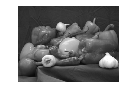
As well, by using RGB2GRAY function as

I = rgb2gray(RGB);

one can convert RGB color image to grayscale image I.

The content of variable I on the workspace is overwritten by the grayscale image of variable RGB.

whos I

  Name        Size              Bytes  Class    Attributes

  I         384x512            196608  uint8

imshow(I)

Applying some operations to image array often requires to convert data into a float type.

For conversion from integer to float, one can use IM2SINGLE or IM2DOUBLE function. These functions convert an image to single and double precision data, respectively.

I = im2double(I);
whos I

  Name        Size               Bytes  Class     Attributes

  I         384x512            1572864  double

The conversion functions to float, i.e., IM2SINGLE function and IM2DOUBLE function, normalizes pixel values to data ranged from 0 to 1.

Verify the minimum and maximum values by using MIN function and MAX function, respectively.

min(I(:))

ans =

    0.0314

max(I(:))

ans =

     1

where the colon index as 'I(:)' victories any array. Function MIN and MAX evaluate each column for array data. Thus, vectorization is applied so that the minimum and maximum value of whole pixels in I are obtained.

A power function can adjust image intensity. Because the pixel values are normalized from 0 to 1, the output values are also lie between the same range.

J = I.^2;
imshow(J)

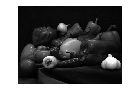
Certify the characteristics of a power function through FPLOT function.

fplot(@(x) x.^2, [0 1])
xlabel('x') % Label for x-axis
ylabel('y') % Label for y-axis
axis square % Adjustment of aspect ratio

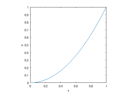
The power function shown here draws parabola and has an effect to darken the image.

[ Top ]

Image Write

By using IMWRITE function, the processed image can be stored as a file.

Write image J to the file named 'darkpeppers.tif.'

imwrite(J,'darkpeppers.tif')

Then, the image is written to file 'darkpeppers.tif.'

dir *.tif

darkpeppers.tif

[ Top ]

Exercises

Exercise 1-1. Intensity Adjustment

Adjust the intensity of the grayscale image of peppers.png by using SQRT function, and then write the result to a TIFF file named 'brightpeppers.tif.' In addition, draw the graph of the conversion function.

(Example Answer)

Exercise 1-2. Color Space Conversion

Convert RGB color array of image file peppers.png to HSV color array by using RGB2HSV function and double the intensity of the S component. Then, return the HSV color array back to RGB color array by using HSV2RGB function. Finally, store the result to a JPEG file named 'highsatpeppers.jpg.'

(Example Answer)

Contents | | Top | | Part2